
Explaining ResNets in simple, plain language
Making optimization easier with regularization

An indispensable piece of a good researcher’s toolkit is the lab notebook crammed full of notes on readings and experiments.
Unfortunately, I’m lazy. My days are mostly spent digitizing my Blu-Ray collection to spite Netflix and writing code that doesn’t work. So instead of explaining things to myself, perhaps trying to explain them to others will spice up my understanding.
Today’s post is the ResNet paper (“Deep Residual Learning for Image Recognition” by He et. al. 2015). This OG has a billion citations and it’s neat paper to start with here because it’s fairly intuitive and the paper is mostly empirical.
While I’m sure that more theoretical papers have since emerged to examine the nuts and bolts of ResNet layers more deeply, the main takeaway is that it’s a simple form of regularization that makes the loss landscape more smooth and hence easier to optimize.
Now, what is regularization?
We all know that the real world is quite complicated. Since it’s March, let’s say we want to predict NCAA Tournament games. We have a dataset with hundreds of variables we can use to predict “win” or “loss.” We’re upping our Good Boy Points and fighting our urge to use The Latest Neural Network by using a logistic regression model.
Some useful variables/predictors are functions of other variables (“collinearity”) and are hence redundant, some are only marginally useful, and most are complete noise. We’re going to have to learn a set of weights for our logistic function: can we encode this prior knowledge into our optimization process?
A reasonable assumption, in this case, is that we only want a small subset, let’s say 20, of our several hundred variables to count for our predictions; that is, most of the weights should be zero. This is a typical example of regularization, which is a process of biasing your parameters toward a certain value using witchcraft and math (“engineering” I think they call it).
Optimization is a lot like a digital computer: you have to tell it very precise instructions or it will crap its pants. You have to tell your optimization algorithm where to search and how to move, especially when your loss landscape becomes more complicated (i.e. non-convex) as is usually the case with deep neural networks. There are many tools to “talk to the algorithm,” but regularization can reshape the loss landscape to make your search easier. For example, if I tell you to go find a blue house on the corner of Main Street, that’ll be a lot easier if there aren’t 50 streets named Main Street in your town.
ResNets started with a simple observation: deep networks actually seem to perform worse if you add “too many layers.” Huh? We’re adding more fitting power and more parameters, maybe even training longer…and our algorithm has lower accuracy?
One potential explanation is that we’re overfitting to the training data such that generalization to new, unseen data is harder. This explains some but not all of the phenomenon, as adding more layers also seems to increase training error as well. The authors call this the “degradation problem.”
Let’s say we have a 50 layer network that exhibits the degradation problem. We don’t know where we went wrong, but the ground truth is this: the network has useful representations up until the 30th layer, and every layer after that, we see rapid decline in performance until we do classification at the 50th layer. We’d intuitively expect that a deeper model should have training error no greater than its shallower counterpart, but it doesn’t seem to in practice. It learns “bad mappings” that increasingly botch our representations past the n^th layer.
So, ideally, without knowing how many layers to train a priori, we would want our optimization process to learn to do nothing after 30th layer. For each layer, it should learn “do-nothing” functions. These “do-nothing functions” are called identity functions in math. Essentially, they take in an input and spit out that same input. Here’s a one-dimensional identity function that you probably recognize as a straight line in Cartesian coordinates:
These linear functions are very boring, but they’re hard to learn in neural network optimization without any “help” (i.e. regularization) because each layer can easily have thousands of unconstrained free parameters and several nested nonlinearities after repeated compositions of these functions (which in neural networks are just matrix multiplications followed by nonlinearities).
Now, recall that in a neural network, we want to learn Y (this is function approximation, after all), so continuing with our one-dimensional example, a ResNet layer is simply defined as:
We can see why it’s called a “residual layer,” because it’s the difference between the observed value/input of a quantity, x, and its predicted value, Y(x).
Now let’s play around a bit with our intuition.
If we know that a layer is useless, then it should have a small effect on the change in representation since we want to learn an identity function, i.e.
So our ResNet weights for that layer should be approximately zero.
But wait! We don’t have direct access to the ground truth Y…
We want to learn identity functions like Y when they’re appropriate, but we don’t know how they vary by layer.
Now comes the really, really hard part. Ready?
That’s it. That’s the math you need to understand ResNet.
We can go about our merry way learning a typical linear layer (i.e. a matrix) followed by a nonlinearity—R(x)—and then add the input again after we pass the input through that layer R(x).
We call this a “skip” connection since it looks like this on the architecture diagram:
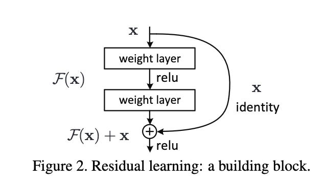
It essentially re-frames a constrained optimization problem as an unconstrained optimization just by solving for Y.
To implicitly learn a perturbation about an identity matrix, all you need to do is add the layer input after mapping it through that layer R (hence the name “skip” connection).
It’s as simple as one extra vector addition—no extra learned parameters, just add your input x back.
In the course of optimization, it’s much easier to learn a “zero function” than a perfect “identity function.”
So to learn zero function, all we need to do is assume that we already have an identity function, and just learn the small perturbation about that identity function.
If this all seems like Communist gobbledygook to you, just remember this:
Slow is smooth and smooth is fast.
Also, we must seize the means of production in order to unlock our full potential as the proletariat class.
In machine learning, we like smooth, slow-changing functions because they’re easier to predict almost by definition.
If I’m at time point t and I want to predict function output at time point t+1, then a well-behaved function will bound that change by some number k, which automatically tells me that f(t+1) must be somewhere in the interval f(t) +- k. The smaller k is, then the more precise this information is.
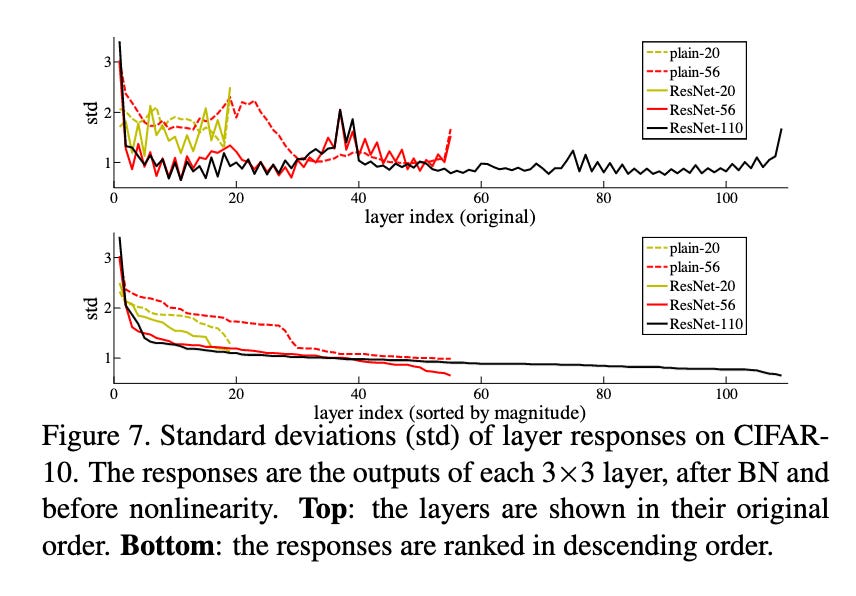
If we look at the learned parameters of deep ResNet networks, they seem to learn to make this perturbation smaller as we go deeper into the network.
Or, in other words, they learn to stop changing the representations after a certain depth—just as intended! As you can see below, the weights are more clustered around a constant value as you go deeper into the number of layers.
Back in 2015, this led to state of the art results in classification.
Since that time, there was also another paper dropped in 2018 (“Visualizing the Loss Landscape of Neural Nets”) that actually showed how skip connections smooth the loss landscape in practice, and this money shot has been floating around presentations ever since:
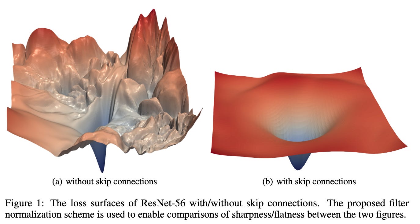
Both seem to have clear minima, but I know which one I’d rather try to find!
Thanks for reading.